It is sometimes overlooked that increasing the sample size will not always reduce the uncertainty in the estimate of a parameter. [1] illustrates this fact as "Misconception 4" with an example considering a random variable having Cauchy distribution. Its probability density function \(f\) has two parameters: \begin{align}f(x;x_0, \gamma) = \frac{1}{\pi \gamma \big[1 + (\frac{x - x_0}{\gamma})^2\big]}\end{align} where \(x_0\) is a real number called the location parameter and \(\gamma (> 0)\) is its scale parameter.
Since the distribution has no (finite) mean, the law of large numbers cannot ensure that taking its sample average converges to \(x_0\). Fortunately it is still possible to estimate \(x_0\) by taking sample median. In fact, the following computational experiment in R code finds sample mean converging to the location parameter quickly:
x <- replicate(16, {
s <- rcauchy(10000, 42)
h <- head(s, 10)
c(median(h), median(s), mean(h), mean(s))
})
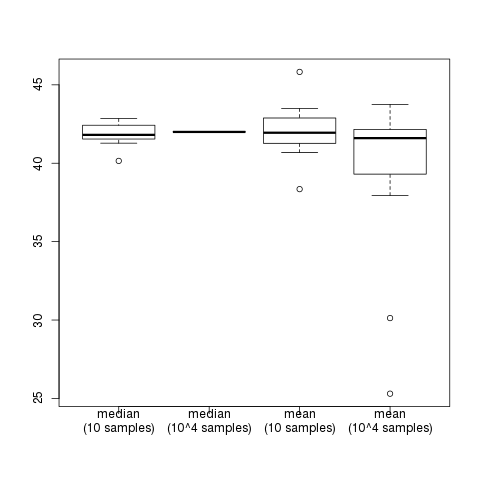
boxplot(t(x), names = c("median\n(10 samples)", "median\n(10^4 samples)", "mean\n(10 samples)", "mean\n(10^4 samples)"))
The resulting figure (obtained with seeding set.seed(1)) shows that the error of sample median from its true value \(42\) is small, while average of 10 samples is more diverse and averaging 10,000 samples often fails in even bigger errors.
Reference: [1] John Kermond, Counterexamples in Probability and Statistics, MAV Annual Conference 2009.